User Guide
The user guide covers the inverse routine and file structure. Users brand new to moment tensor inversion should check out the Jupyter Notebook tutorials for an complete example that includes data processing and synthetics calculation.
Further information on any specific method can be obtained in the API Reference.
Basics
The inverse routine is divided into three main parts:
Parsing an input file to get a set of parameters required to run the inversion.
Perform the inversion based on the parameters provided.
Write the results to file.
>>> # import the package
>>> import mttime

>>> # 1. read input file and set up the inversion
>>> config = mttime.Configure(path_to_file="mtinv.in")
>>> mt = mttime.Inversion(config=config)

>>> # 2. Run inversion and plot the result (if plotting function is turned on)
>>> mt.invert()

>>> # 3. Save result to file
>>> mt.write()
We will go over the details in the following sections.
Dataset
In this section we will introduce the file structure and input parameters using an example. The earthquake in this example occured near Byron, California on July 16, 2019. The raw data and instrument response were obtained from the IRIS DMC using ObsPy’s mass_downloader functionality.
Directory and file structures
In this example all of the files (input, data and synthetics) are assumed to be located under a single root directory called project:
project
|    mtinv.in
|
|____40191336
|    |  BK.QRDG.00.z.dat
|    |  BK.RUSS.00.z.dat
|    |  ...
|
|____40191336/gil7
     |  BK.QRDG.00.12.0000.ZDD
     |  BK.QRDG.00.12.0000.ZDS
     |  ...
Under project there is the input parameter file mtinv.in which contains headers and a station table:
origin         2019-07-16T20:11:01.470000Z
longitude      -121.7568
latitude       37.8187
depth          10,12,20
path_to_data   40191336
path_to_green  40191336/gil7
green          herrmann
components     ZRT
degree         6
weight         distance
plot           1
correlate      0
    station  distance  azimuth  ts  npts   dt  used  longitude  latitude
 BK.QRDG.00     80.99   335.29  32   150 1.00     1    -122.14     38.48
 BK.RUSS.00     81.16   353.18  32   150 1.00     1    -121.87     38.54
  BK.CVS.00     84.88   313.73  31   150 1.00     1    -122.46     38.35
 BK.OAKV.00     88.89   320.02  31   150 1.00     1    -122.41     38.43
 BK.FARB.00    110.46   263.41  31   150 1.00     1    -123.00     37.70
  BK.SAO.00    120.23   166.71  31   150 1.00     1    -121.45     36.76
  BK.CMB.00    122.83    78.33  31   150 1.00     1    -120.39     38.03
 BK.MNRC.00    132.06   333.21  32   150 1.00     1    -122.44     38.88
Configure object will parse the input
text file.
>>> config = mttime.Configure(path_to_file="mtinv.in")
The headers have two columns: a parameter name and its corresponding value. If the values are left blank, the default values will be used instead. A descrption of the parameters are shown here:
parameters |
description |
|---|---|
path_to_file |
path to input file containing headers and station information.
Directory will become the project root directory. Default is |
datetime |
event origin time, optional. |
longitude |
event longitude, optional. |
latitude |
event latitude, optional. |
depth |
source depths to invert. |
path_to_data |
path to data files, relative to root directory.
Defaults is |
path_to_green |
path to Green’s function files, relative to root directory.
Defaults is |
green |
Green’s function format, options are |
components |
waveform components, options are |
degree |
degrees of freedom allowed in the inversion, options are |
weight |
data weights, options are |
plot |
If |
correlate |
Flag to cross-correlate data and Green’s functions
for best time shift in time points. Default is |
Station table
Lines 13 and onward in mtinv.in contain the station information, line 13 is the station header and should not be modified. A description of the headers is shown here:
headers |
description |
|---|---|
station |
file names of data and synthetics |
distance |
source-receiver distance |
azimuth |
source-receiver azimuth |
ts |
shift data by the number of time points specified |
npts |
number of samples to invert |
dt |
sampling interval in seconds |
used |
components to invert, set 1 to invert and 0 for prediction only. For three component data you can set flags for individual components, ordered by ZRT. e.g. 110 will invert ZR components only |
longitude |
station longitude |
latitude |
station latitude |
Waveform Data
mttime expects both observed and synthetic Green’s functions to be fully processed. This means they are corrected for instrument response, filtered, and decimated, and saved as SAC binary files.
The data file names have the following format:
[station].[component].dat
station: from the station column
component: Z, R, or T (from the components parameter)
With the example above the data file names for station BK.CMB.00 are:
BK.CMB.00.Z.dat
BK.CMB.00.R.dat
BK.CMB.00.T.dat
Synthetic Seismograms
The basis Green’s functions can be combined to create three component time histories for an arbitrarily oriented
point source. As mentioned previously two types of synthetic basis Green’s functions are accepted:
herrmann and tensor.
The tensor format is pretty straight forward, it consists of the six elementary tensor elements in cartesian space. north, east and down directions (x, y and z) in Aki and Richards (2002). The herrmann format is based on the formulation of Herrmann and Wang (1985), which consists of ten fundamental source types.
The synthetic file names have the following format:
[station].[depth].[green_function_name]
station: from the station column
depth: source depth with four significant digits
component: Z, R, or T (from the components parameter)
green_function_name: this depends on format of the Green’s functions
herrmann: TSS, TDS, RSS, RDS, RDD, ZSS, ZDS, ZDD, REX, and ZEX (total of 10)tensor: ZXX, ZYY, ZZZ, ZXY, ZXZ, ZYZ, RXX, etc. (total of 18)
With the example above the synthetic file names for station BK.CMB.00 are:
BK.CMB.00.12.0000.TSS
BK.CMB.00.12.0000.TDS
and so on.
If we change the format to tensor (such that green="tensor"), the file names become:
BK.CMB.00.12.0000.TXX
BK.CMB.00.12.0000.TXY
and so on.
Output Files
Running the inversion with the example above will generate the following outputs.
>>> mt = mttime.Inversion(config=config)
>>> mt.invert()
>>> mt.write()
Text files:
d10.0000.mtinv.out - moment tensor solution at 10 km depth
d12.0000.mtinv.out
d20.0000.mtinv.out
Full Moment Tensor Inversion
Depth = 10.0000 (km)
Mo = 3.833e+22 (dyne-cm)
Mw = 4.36
Percent DC   =  90
Percent CLVD =   8
Percent ISO  =   3
Fault Plane 1: Strike=233 Dip=66 Rake=-6
Fault Plane 2: Strike=326 Dip=84 Rake=-156
Percent Variance Reduction = 74.47

Moment Tensor Elements: Aki and Richards Cartesian Coordinates
Mxx        Myy        Mzz        Mxy        Mxz        Myz
-2.836e+22 3.458e+22  -3.037e+21 -1.067e+22 1.033e+22  1.066e+22

Harvard/CMT convention
Mrr        Mtt        Mpp        Mrt        Mrp        Mtp
-3.037e+21 -2.836e+22 3.458e+22  1.033e+22  -1.066e+22 1.067e+22

Eigenvalues: 3.833e+22 -3.790e+20 -3.477e+22
Lune Coordinates: -1.95  2.03
Station Information
    station distance azimuth  ts  npts   dt  Z  R  T weights    VR longitude latitude
 BK.QRDG.00    80.99  335.29  32   150 1.00  1  1  1    1.00 89.26  -122.140   38.480
 BK.RUSS.00    81.16  353.18  32   150 1.00  1  1  1    1.00 73.30  -121.870   38.540
  BK.CVS.00    84.88  313.73  31   150 1.00  1  1  1    1.05 74.81  -122.460   38.350
 BK.OAKV.00    88.89  320.02  31   150 1.00  1  1  1    1.10 32.40  -122.410   38.430
 BK.FARB.00   110.46  263.41  31   150 1.00  1  1  1    1.36 56.80  -123.000   37.700
  BK.SAO.00   120.23  166.71  31   150 1.00  1  1  1    1.48 86.32  -121.450   36.760
  BK.CMB.00   122.83   78.33  31   150 1.00  1  1  1    1.52 85.93  -120.390   38.030
 BK.MNRC.00   132.06  333.21  32   150 1.00  1  1  1    1.63 82.31  -122.440   38.880
Figures:
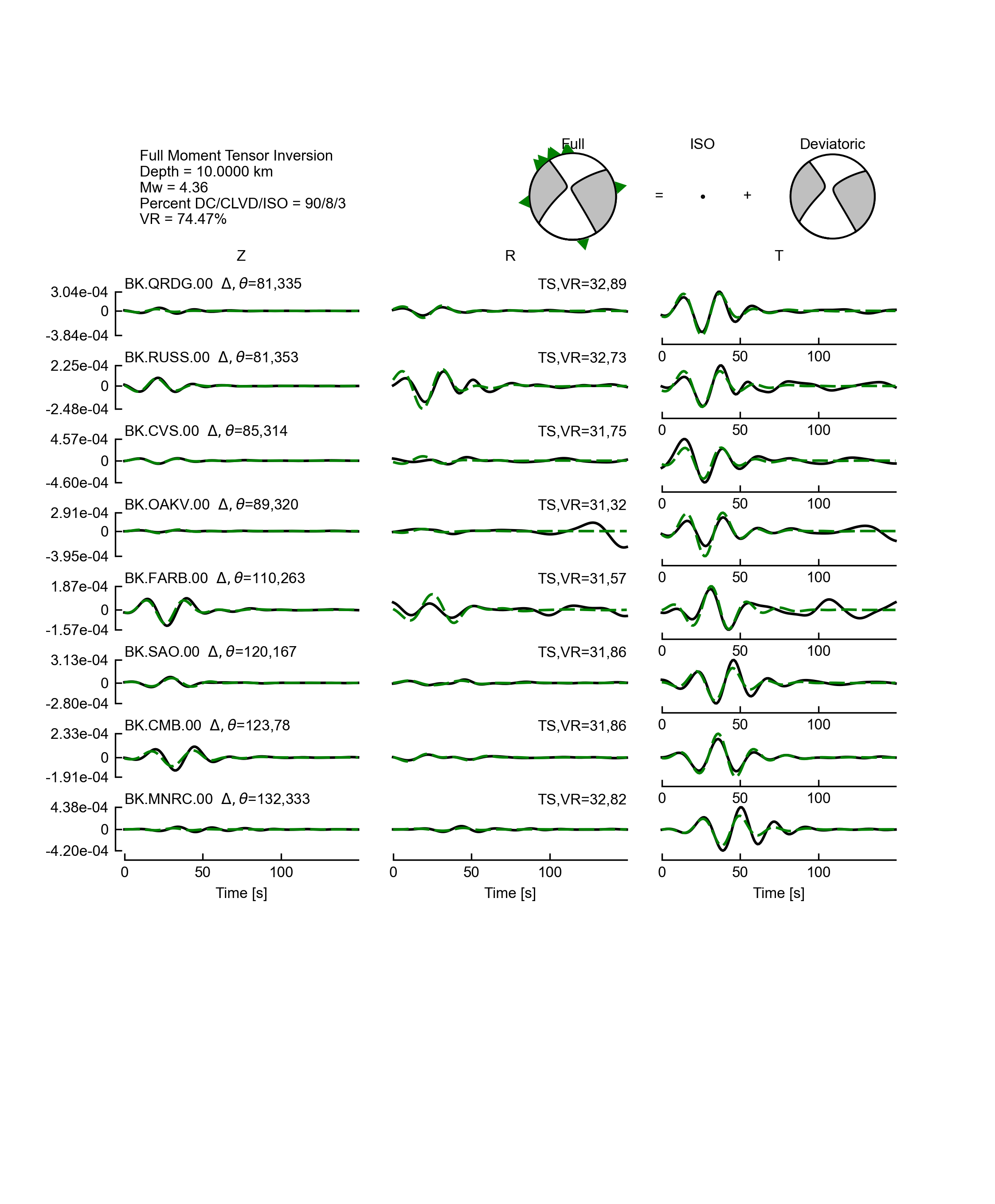
bbwaves.d10.0000.00.eps - focal mechanism and waveform fits at 10 km depth
bbwaves.d12.0000.00.eps
bbwaves.d20.0000.00.eps
depth.bbmw.eps
Since we performed the inversion at multiple source depths, in addition to the standard focal mechanism and waveform figures, the plotting function will also generate a figure that shows the solution as function of source depth.
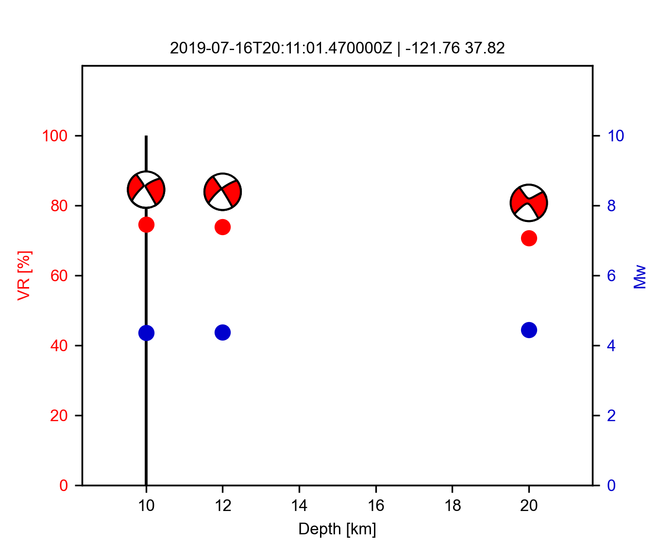
Figure Options
There are more display options available in
mttime.core.inversion.Inversion.plot.
view="waveform"- MT solution and waveform fits.
view="depth"- MT solution as a function of source depth.
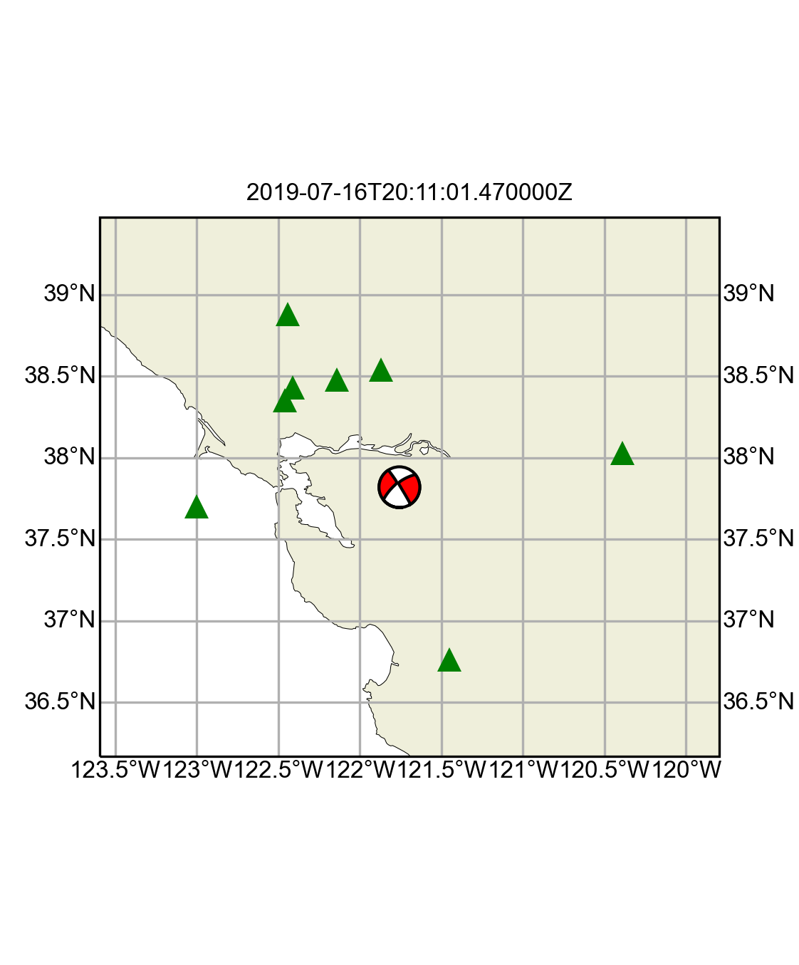
view="map"- map view.
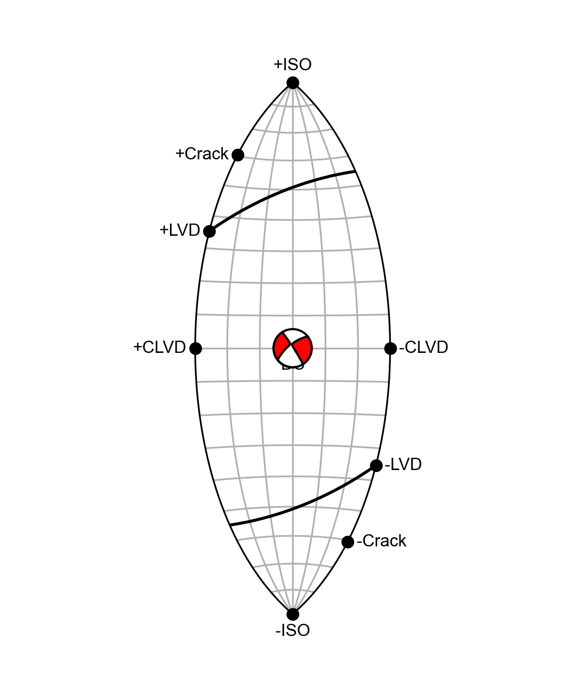
view="lune"- full MT source-type on the lune.
In the example above we set mt.config.plot=True, which is equivalent to:
>>> mt.plot(view="waveform")
>>> mt.plot(view="depth") # if depth is not fixed
To plot the solution on a map or lune:
>>> mt.plot(view="map", show=True)
>>> mt.plot(view="lune", show=True)